Get Started

In this vignette, you will learn everything you need to know to get started implementing numerical algorithms using {anvil}. If you have experience with JAX in Python, you should feel right at home.

The `AnvilTensor`

We will start by introducing the main data structure, which is the AnvilTensor. It is essentially like an R array, with some differences:

It supports more data types, such as different precisions, as well as unsigned integers.
The tensor can live on different devices, such as CPU or GPU.
0-dimensional tensors can be used to represent scalars.

We can create an AnvilTensor from R objects using nv_tensor. Below, we create a 0-dimensional tensor (i.e., a scalar) that holds a 16-bit integer on the CPU.

library(anvil)
set.seed(42)
nv_tensor(1L, dtype = "i16", device = "cpu", shape = integer())

## AnvilTensor 
##  1
## [ CPUi16{} ]

Note that for the creation of scalars, you can also use nv_scalar as a shorthand to skip specifying the shape and omit specifying the device, as CPU is the default.

nv_scalar(1L, dtype = "i16")

## AnvilTensor 
##  1
## [ CPUi16{} ]

We can also create higher-dimensional tensors, for example a 2x3 tensor with single-precision floating-point numbers. Without specifying the data type, it will default to "f32" for R doubles and "i32" for integers.

x <- array(1:6, dim = c(2, 3))
y <- nv_tensor(x)
y

## AnvilTensor 
##  1 3 5
##  2 4 6
## [ CPUi32{2x3} ]

The as_array() function allows to convert AnvilTensors back to R objects. Note that for 0-dimensional tensors, the result is an R vector of length 1, as R arrays cannot have 0 dimensions.

as_array(y)

##      [,1] [,2] [,3]
## [1,]    1    3    5
## [2,]    2    4    6

At first, working with AnvilTensors may feel a bit cumbersome, because you cannot directly apply functions to them like you would with regular R arrays.

x + x

##      [,1] [,2] [,3]
## [1,]    2    6   10
## [2,]    4    8   12

y + y

## i32{2,3}

JIT Compilation

In order to work with AnvilTensors, you need to convert the function you want to apply to a jit-compiled version via jit().

plus_jit <- jit(`+`)
plus_jit(y, y)

## AnvilTensor 
##   2  6 10
##   4  8 12
## [ CPUi32{2x3} ]

The result of the operation is again an AnvilTensor.

We can also jit-compile more complex functions. Below, we define a function that takes in a data matrix X, a weight vector beta, and a scalar bias alpha, and computes the linear model output \(y = X \times \beta + \alpha\).

linear_model_r <- function(X, beta, alpha) {
  X %*% beta + alpha
}

linear_model <- jit(linear_model_r)

X <- nv_tensor(rnorm(6), dtype = "f32", shape = c(2, 3))
beta <- nv_tensor(rnorm(3), dtype = "f32", shape = c(3, 1))
alpha <- nv_scalar(rnorm(1), dtype = "f32")

linear_model(X, beta, alpha)

## AnvilTensor 
##   2.7911
##  -1.1904
## [ CPUf32{2x1} ]

One restriction of {anvil} is that a function has to be re-compiled for every unique combination of input types, each consisting of a specific shape and data type. To demonstrate this, we create a slightly modified version of our previous linear predictor function:

linear_model2 <- jit(function(X, beta, alpha) {
  cat("compiling ...\n")
  X %*% beta + alpha
})

Next, we create a little helper function that creates example inputs with different numbers of observations:

simul_data <- function(n, p) {
  list(
    X = nv_tensor(rnorm(n * p), dtype = "f32", shape = c(n, p)),
    beta = nv_tensor(rnorm(p), dtype = "f32", shape = c(p, 1)),
    alpha = nv_scalar(rnorm(1), dtype = "f32")
  )
}

Below, we call the function twice on data with the same shapes.

do.call(linear_model2, simul_data(2, 3))

## compiling ...

## AnvilTensor 
##   4.9640
##  -0.1413
## [ CPUf32{2x1} ]

do.call(linear_model2, simul_data(2, 3))

## AnvilTensor 
##   0.6140
##  -2.5214
## [ CPUf32{2x1} ]

We can notice that we only see the "compiling ..." message the first time, where the function is first compiled into an XLA executable, cached, and executed. The second time, the executable is retrieved from the cache (because the inputs have the same shapes and data types) and executed without recompilation. Because the executable contains only the operations applied to AnvilTensors, it does not contain the cat() call, so we don’t see it the second time.

If we call the function on data with different shapes (or data types), the function is re-compiled and the message re-appears.

y_hat <- do.call(linear_model2, simul_data(4, 3))

## compiling ...

Because the compilation step itself can take some time, {anvil} therefore gives the best results when the same function is called many times with the same (or only a few different) input types, or the computation itself is sufficiently large to amortize the compilation overhead.

Static Arguments

Besides AnvilTensors, jit-compiled functions can also take in regular R values as arguments. For example, we might want a linear model with or without a bias term. To do so, we add the logical(1) argument with_bias to our function. We need to mark this argument as static, so {anvil} knows to treat it as a regular R value.

linear_model3 <- jit(function(X, beta, alpha = NULL, with_bias) {
  if (with_bias) {
    cat("Compiling with bias ...\n")
    X %*% beta + alpha
  } else {
    cat("Compiling without bias ...\n")
    X %*% beta
  }
}, static = "with_bias")

We can now call this function with or without a bias term:

linear_model3(X, beta, with_bias = FALSE)

## Compiling without bias ...

## AnvilTensor 
##   2.8538
##  -1.1277
## [ CPUf32{2x1} ]

linear_model3(X, beta, alpha, with_bias = TRUE)

## Compiling with bias ...

## AnvilTensor 
##   2.7911
##  -1.1904
## [ CPUf32{2x1} ]

Static arguments work differently than AnvilTensors as the function will be re-compiled for each new observed value of the static argument, not only each unique input type combination.

Nested Inputs and Outputs

Inputs and outputs can also be nested data structures that contain AnvilTensors, although we currently only support (named) lists.

linear_model4 <- jit(function(inputs) {
  list(y_hat = inputs[[1]] %*% inputs[[2]] + inputs[[3]])
})
linear_model4(list(X, beta, alpha))

## $y_hat
## AnvilTensor 
##   2.7911
##  -1.1904
## [ CPUf32{2x1} ]

So far, we have only implemented the prediction step for the linear model. One of the core applications of {anvil} is to implement learning algorithms, for which we often need gradients, as well as control flow. We will start with gradients.

Automatic Differentiation

In {anvil}, you can easily obtain the gradient function of a scalar-valued function via gradient(). Currently, we don’t support jacobians or hessians, but this will hopefilly be added in the future. Below, we implement the loss function for our linear model.

mse <- function(y_hat, y) {
  mean((y_hat - y)^2.0)
}

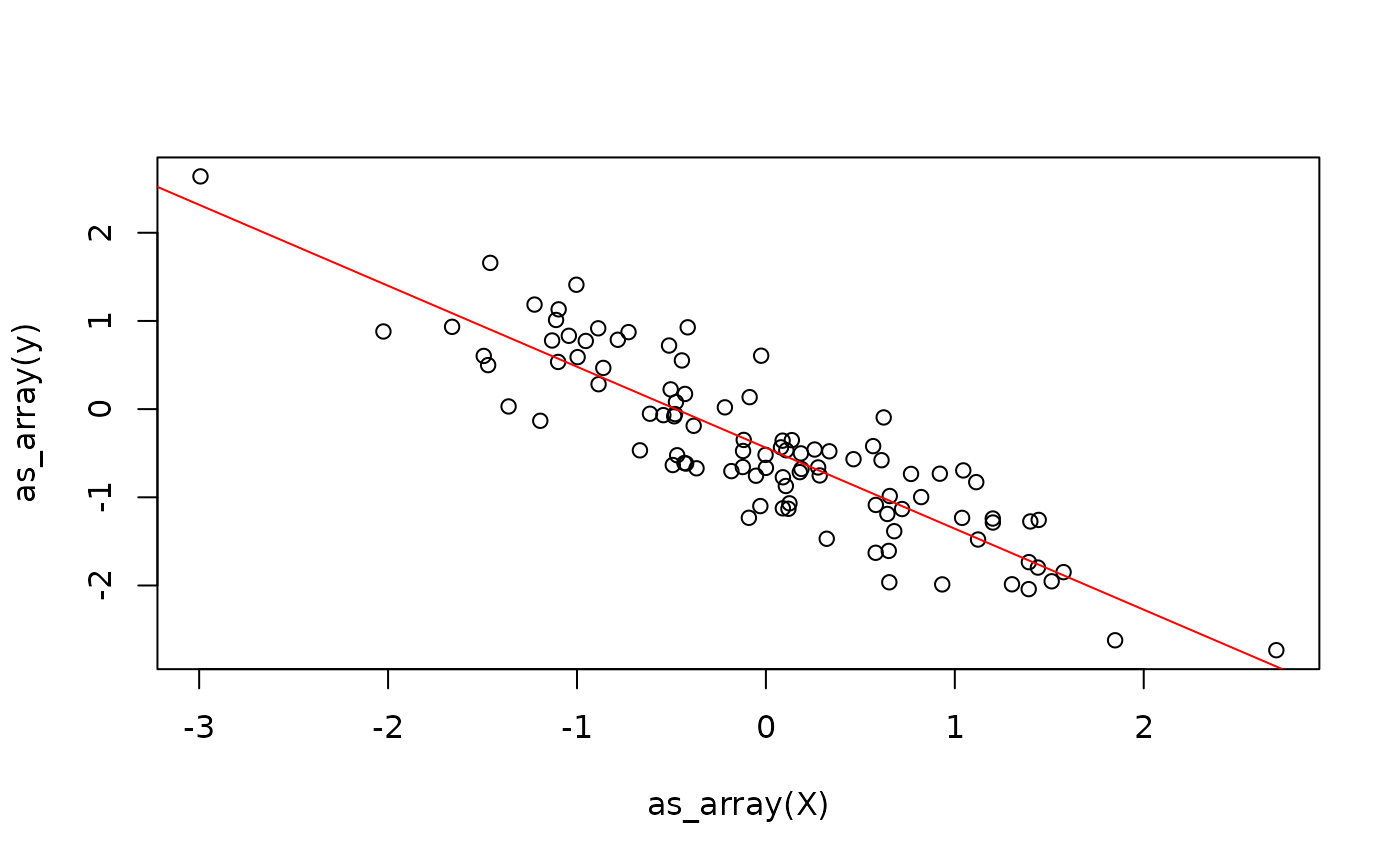
We now need some target variables y, so we simulate some data from a linear model:

beta <- rnorm(1)
X <- matrix(rnorm(100), ncol = 1)
alpha <- rnorm(1)
y <- X %*% beta + alpha + rnorm(100, sd = 0.5)
plot(X, y)

X <- nv_tensor(X)
y <- nv_tensor(y)

Next, we randomly initialize the model parameters:

beta_hat <- nv_tensor(rnorm(1), shape = c(1, 1), dtype = "f32")
alpha_hat <- nv_scalar(rnorm(1), dtype = "f32")

We can now define a function that does the prediction and calculates the loss. Note that we are calling into the original R function that does the prediction and not its jit-compiled version.

model_loss <- function(X, beta, alpha, y) {
  y_hat <- linear_model_r(X, beta, alpha)
  mse(y_hat, y)
}

Using the gradient() transformation, we can automatically obtain the gradient function of model_loss with respect to some of its arguments, which we specify.

model_loss_grad <- gradient(
  model_loss,
  wrt = c("beta", "alpha")
)

Finally, we define the update step for the weights using gradient descent.

update_weights_r <- function(X, beta, alpha, y) {
  lr <- 0.1
  grads <- model_loss_grad(X, beta, alpha, y)
  beta_new <- beta - lr * grads$beta
  alpha_new <- alpha - lr * grads$alpha
  list(beta = beta_new, alpha = alpha_new)
}
update_weights <- jit(update_weights_r)

This already allows us to fit the linear model

weights <- list(beta = beta_hat, alpha = alpha_hat)
for (i in 1:100) {
  weights <- update_weights(X, weights$beta, weights$alpha, y)
}

While this might seem like a reasonable solution, it continuously switches between the R interpreter and the XLA runtime. Moreover, we allocate new tensors in each iteration for the weights. While the latter might not be a big problem for small models, it can cause significant overhead when working with bigger tensors.

Next, we will discuss control flow in {anvil} before we address immutability.

Control Flow

In principle, there are three ways to implement control-flow in {anvil}:

Embed jit-compiled functions inside R control-flow constructs, which we have seen earlier.
Embed R control flow inside a jit-compiled function (we have also seen this earlier when our linear model allowed to optionally include a bias term).
Use special control-flow primitives provided by anvil, such as nv_while() and nv_if().

Which solution is best depends on the specific scenario, so we will cover all three cases, at the risk of being a bit repetitive. We will illustrate this with our linear model training example from earlier. The first implementation is what we have already seen earlier: we jit-compile the update step and then repeatedly call it in an R loop:

n_steps <- 100L
beta_hat <- nv_tensor(rnorm(1), shape = c(1, 1), dtype = "f32")
alpha_hat <- nv_scalar(rnorm(1), dtype = "f32")

weights <- list(beta = beta_hat, alpha = alpha_hat)
for (i in seq_len(n_steps)) {
  weights <- update_weights(X, weights$beta, weights$alpha, y)
}
weights

## $beta
## AnvilTensor 
##  -0.9184
## [ CPUf32{1x1} ] 
## 
## $alpha
## AnvilTensor 
##  -0.4376
## [ CPUf32{} ]

For simple update steps, this solution can be inefficient because every call into a jit-compiled function has some overhead. How significant this overhead is depends on how expensive each call in the loop is – for expensive functions the overhead becomes negligible.

The second approach is to use an R loop within the jit-compiled function. There, the loop will be unrolled during the compilation step (for conditionals, only one branch is included in the executable as discussed earlier). This will be rather slow in the example at hand, because we will also re-compute the gradient function in each iteration. Moreover, the parameter n_steps is static, which means that for every unique value of n_steps, the function will be re-compiled into a different executable.

train_unrolled <- jit(function(X, beta, alpha, y, n_steps) {
  lr <- nv_scalar(0.1)
  for (i in seq_len(n_steps)) {
    grads <- model_loss_grad(X, beta, alpha, y)
    beta <- beta - lr * grads$beta
    alpha <- alpha - lr * grads$alpha
  }
  list(beta = beta, alpha = alpha)
}, static = "n_steps")

beta_hat <- nv_tensor(rnorm(1), shape = c(1, 1), dtype = "f32")
alpha_hat <- nv_scalar(rnorm(1), dtype = "f32")
train_unrolled(X, beta_hat, alpha_hat, y, n_steps = 10L)

## $beta
## AnvilTensor 
##  -0.9600
## [ CPUf32{1x1} ] 
## 
## $alpha
## AnvilTensor 
##  -0.3703
## [ CPUf32{} ]

Finally, the third approach is to use the nv_while function. It is not like a standard while loop, because anvil is purely functional.

The function takes in:

An initial state, which is a (nested) list of AnvilTensors.
A cond function, which takes as input the current state and returns a logical flag indicating whether to continue the loop.
A body function, which takes as input the current state and returns a new state.

train_while <- jit(function(X, beta, alpha, y, n_steps) {
  lr <- 0.1
  nv_while(
    list(beta = beta, alpha = alpha, i = nv_scalar(0L)),
    \(beta, alpha, i) i < n_steps,
    \(beta, alpha, i) {
      grads <- model_loss_grad(X, beta, alpha, y)
      list(
        beta = beta - lr * grads$beta,
        alpha = alpha - lr * grads$alpha,
        i = i + 1L
      )
    }
  )
})

beta_hat <- nv_tensor(rnorm(1), shape = c(1, 1), dtype = "f32")
alpha_hat <- nv_scalar(rnorm(1), dtype = "f32")
train_while(X, beta_hat, alpha_hat, y, nv_scalar(100L))

## $beta
## AnvilTensor 
##  -0.9184
## [ CPUf32{1x1} ] 
## 
## $alpha
## AnvilTensor 
##  -0.4376
## [ CPUf32{} ] 
## 
## $i
## AnvilTensor 
##  100
## [ CPUi32{} ]

The same approach works analogously for if-statements, where the {anvil} primitive nv_if is available.

Immutability

AnvilTensor objects are immutable, i.e., once created, their value cannot be changed. In other words, there are conceptually no in-place updates like x[1] <- x[1] + 1. This means that {anvil} follows value semantics, i.e., functions are pure. Naturally, this raises the question of how this impacts performance. We need to distinguish two scenarios:

Updating an AnvilTensor that “lives within” a jit-compiled function.
Updating an AnvilTensor “living in R” through a jit-compiled function.

For the first scenario, there is nothing to worry about. The XLA compiler is able to optimize this, ensuring that no unnecessary copies are actually made. This is similar to copy-on-write semantics in R. If you evaluate x <- 1:10; y <- x, you are conceptually creating a copy of x when assigning it to y, but internally, this is optimized away and the copy will only be created when modifying y or x. Because {anvil} uses compilation and shapes are known at compile time, it can make many more such optimizations, minimizing unnecessary copies as much as possible.

However, there is also the case where one calls into an {anvil} function from R code, as we have done in our initial linear model example.

weights <- update_weights(X, weights$beta, weights$alpha, y)

Because the assignment of the outputs of the {anvil} function to R variables does not happen within the executable, the XLA compiler cannot optimize this. If we know that some of the inputs to the {anvil} function are not needed anymore after the function call (as is the case for “update-calls” like above), we can mark them as “donatable” when jit-compiling.

update_weights_donatable <- jit(update_weights_r, donate = c("beta", "alpha"))

This will tell the XLA compiler that we no longer need the inputs alpha and beta afterwards, so their underlying memory can be reused.

weights_out <- update_weights_donatable(X, weights$beta, weights$alpha, y)

If we now print the input weights, we get an error because the tensors have been deleted.

weights

## $beta
## AnvilTensor

## Error:
## ! ToLiteral() called on deleted or donated buffer: INVALID_ARGUMENT: Buffer has been deleted or donated.

But the new weights are still there.

weights_out

## $beta
## AnvilTensor 
##  -0.9184
## [ CPUf32{1x1} ] 
## 
## $alpha
## AnvilTensor 
##  -0.4376
## [ CPUf32{} ]